Old habits

Or: Recombination dynamics in a coupled two-level system with strong nonradiative contribution (an ipython notebook)

One of my students investigates the transient behavior of the photoluminescence emitted by (In,Ga)N quantum heterostructures after being irradiated by a short laser pulse. The characteristic feature of the transients he observes for these structures is a power-law decay of the photoluminescence intensity with time at low temperatures (10 K), which changes into an exponential decay at higher temperatures (150 K).

His results reminded me of ones I acquired myself ages ago, during my own time as a PhD student. I didn't have a sensible interpretation then, but I do have one now. Hence, to the surprise of my student, I nonchalantly wrote down the following two coupled differential equations as if they had just occurred to me:

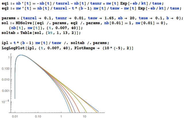
${\dot n_b} = -n_b/\tau_{rel} - n_b/\tau_{nr} + n_w \exp(-\frac{E_b}{k_B T})/\tau_e$

${\dot n_w} = n_b/\tau_{rel} - t^{b-1} n_w/\tau_{w} - n_w \exp(-\frac{E_b}{k_B T})/\tau_e$

with the second term in the second equation ($t^{b-1} n_w/\tau_{w}$) being the experimental observable. The form of this term is giving rise to what is known as a stretched exponential, which for $b \rightarrow 0$ approaches a power law for long times.

Using Mathematica, it takes 7 lines of code to solve this system and to plot it for several temperatures $T$ (or, equivalently and as done here, for different energies $k_B T$):

from IPython.display import Image
Image(filename='/home/cobra/ownCloud/MyStuff/Documents/pdes-net.org/files/images/deqs.png')

As I had hoped, this simple model reproduces the behavior observed in the experiment fairly well. My student was also pleased, but only with the result, not with the method: he's familiar with Matlab, but not with Mathematica. Well, I suspect that he's also not too familiar with Matlab, since he could otherwise have easily solved the equations himself.

In any case, his admission reminded me that I actually wanted to migrate my computational activities to free software whenever possible. It's not easy to get rid of old habits, and as I'm using Mathematica since 23 years, the code above just came naturally, while the one below still required an explicit intellectual effort. But that's essentially the same lame excuse which I'm tired to hear from users of, for example, Microsoft Office when asked to prepare a document with LibreOffice.

So let's get moving. Here's the above differential equation system solved and plotted using numpy, scipy, and matplotlib in an ipython notebook. Note how the notebook integrates the actual code with comments, links, pictures and equations. Editing this notebook is a real treat thanks to the use of markdown and LaTeX syntax.

#Initialize
%matplotlib inline
import matplotlib as mpl
import matplotlib.pyplot as plt
import numpy as np
from scipy.integrate import odeint 

mpl.rcParams['figure.figsize'] = (6, 4)
mpl.rcParams['font.size'] = 16
mpl.rcParams['text.usetex'] = True
mpl.rcParams['font.family'] = 'Serif'
mpl.rcParams['lines.linewidth'] = 2
mpl.rcParams['xtick.major.pad'] = 7

# Parameters
taurel = 0.1       # capture time
taue = 0.1         # emission time
taunr = 0.01       # nonradiative lifetime
tauw = 1.65        # radiative lifetime
eb = 20            # activation energy (in meV)
b = 0              # stretching parameter (approaches power law for b -> 0)

# solve the system dn/dt = f(n,t) and plot the solution
fig = plt.figure()
#for kt in np.linspace(1,13,7):          # approximate temperatures
for T in [10,30,50,70,100,150]:          # exact temperatures

    kt = 0.086173324*T                   # in meV

    def f(n,t):
            nbt = n[0]
            nwt = n[1]
            # the model equations
            f0 = - nbt/taurel - nbt/taunr + nwt*np.exp(-eb/kt)/taue
            f1 = nbt/taurel - nwt*np.exp(-eb/kt)/taue - t**(b-1)*nwt/tauw
            return [f0, f1]

    # initial conditions
    nb0 = 1.                            # initial population in barrier
    nw0 = 0                             # initial population in well
    n0 = [nb0, nw0]                     # initial condition vector
    t  = np.logspace(-2,2,1000)         # logarithmic time grid

    # solve the DES
    soln = odeint(f, n0, t)
    nb = soln[:, 0]
    nw = soln[:, 1]

    # plot results
    plt.loglog(t, t**(b-1)*nw/tauw/max(t**(b-1)*nw/tauw), label=r'%.0f K' %T)
    plt.xlabel('Time (ns)')
    plt.ylabel('Intensity (arb. units)')
    plt.axis([7e-3,40,1e-5,2]);
    plt.legend(loc='lower left', frameon=False, prop={'size':15}, labelspacing=0.15)

fig.savefig('transients.pdf')

The above command saves this plot as a publication-ready figure in pdf format. There are many other available formats, including eps (for the traditional LaTeX/dvipdf toolchain), svg (for further editing with inkscape, or publishing in the web) and png (for insertion in a Powerpoint/Impress presentation).